



Most pre‑buy spreadsheets fail for the same boring reason: they compare the unit discount against nothing. The buyer sees "12% off at 2,000 units" and the math stops there. Then three months later the warehouse is jammed, two split shipments cost a freight premium nobody modeled, and a third of the lot is sitting in a corner that someone will eventually write down.
This is the opposite of that. It's a tight, copy‑paste layout you can drop into Google Sheets or Excel today to compare three strategies — buy‑now‑full, split‑buy (two or three tranches), and buy‑as‑needed — with every ugly cost line included: per‑order receiving cost, per‑unit handling labor, freight premium on split orders, an obsolescence reserve, and a capital‑carry line that actually reflects what the cash costs you.
If you want the strategy‑level reasoning behind split buys, the compact seasonal pre‑buy playbook covers the tactics. This post is the calculator that sits underneath it.
The spreadsheet layout (exact tabs, rows and columns)
Build three tabs: Inputs, Compare, and Sensitivity. Keep all your assumptions on Inputs so you never hunt for a hardcoded number buried in a formula.
Tab 1: Inputs
Put labels in column A, values in column B. Use these exact cell addresses so the formulas below paste cleanly.
| Cell | Label | Example value |
|---|---|---|
| B1 | Annual demand (units) | 6,000 |
| B2 | Base unit cost (no discount) | 9.40 |
| B3 | Pre‑buy discount % (full buy) | 0.12 |
| B4 | Pre‑buy discount % (split buy) | 0.07 |
| B5 | Units per pallet | 480 |
| B6 | Pallet storage cost ($/pallet/month) | 28 |
| B7 | Receiving cost per order ($) | 65 |
| B8 | Handling labor per unit ($) | 0.18 |
| B9 | Freight per standard order ($) | 340 |
| B10 | Freight premium per split order ($) | 120 |
| B11 | Annual capital cost rate (your real cost of cash) | 0.14 |
| B12 | Obsolescence reserve % | 0.05 |
| B13 | Number of orders — full buy | 1 |
| B14 | Number of orders — split buy | 3 |
| B15 | Number of orders — buy‑as‑needed | 12 |
| B16 | Avg months inventory sits (full buy) | 6 |
| B17 | Avg months inventory sits (split buy) | 2.5 |
| B18 | Avg months inventory sits (buy‑as‑needed) | 0.75 |
A quick note on B11, because it's the line most people fudge. If you're financing inventory on a line of credit, use the actual APR. If you're paying cash, use your realistic opportunity cost — what that cash would earn or save elsewhere. A lot of SMBs still run their models at a lazy 8% while their LOC is sitting at 13–15%. That gap quietly makes every big pre‑buy look better than it actually is.
Converting pallet (or cube) costs to $/unit/month
Storage quotes almost never come in the unit you actually plan with. You get a pallet rate, or a cubic‑foot rate from a 3PL, and then nobody converts it — so storage gets left out of the comparison entirely.
Never run out of stock or overorder again.
Listoly streamlines inventory workflows to keep your business stocked and profitable.
- Real-time stock tracking
- Automated reorder alerts
- Supplier and purchase management
No credit card required
Pallet → $/unit/month:
=B6/B5
That's pallet storage cost divided by units per pallet. With the example numbers: 28 / 480 = $0.0583 per unit per month.
If your 3PL quotes by cube instead, add two rows: cube per unit (B19) and cost per cube per month (B20), then:
=B20*B19
So a unit at 0.35 cubic feet in a facility charging $0.90/cube/month costs 0.90 * 0.35 = $0.315 per unit per month. Notice how different that is from the pallet number — cube pricing punishes bulky low‑value items hard, and that's exactly the SKU people tend to over‑buy. Run both if you have both quotes.
Put your chosen storage rate in B21 (call it "Storage $/unit/month") so the Compare tab points to one clean cell.
Tab 2: Compare — the full formula set
Lay out three columns: C = Full buy, D = Split buy, E = Buy‑as‑needed. Labels down column B.
Here are the rows and the exact copy‑paste formulas. Everything references the Inputs tab (assumed named Inputs).
Row — Units purchased (annual): same demand across all three.
-
C
=Inputs!B1 -
D
=Inputs!B1 -
E
=Inputs!B1
Row — Effective unit cost after discount:
-
C
=Inputs!B2*(1-Inputs!B3) -
D
=Inputs!B2*(1-Inputs!B4) -
E
=Inputs!B2
Row — Product cost (annual):
-
C
=C[units]*C[effective unit cost] -
D
=D[units]*D[effective unit cost] -
E
=E[units]*E[effective unit cost]
(Replace the bracketed references with the actual cell addresses in your sheet — e.g. =C3*C4.)
Row — Receiving cost (annual):
-
C
=Inputs!B7*Inputs!B13 -
D
=Inputs!B7*Inputs!B14 -
E
=Inputs!B7*Inputs!B15
Row — Handling labor (annual):
-
C
=Inputs!B8*C[units] -
D
=Inputs!B8*D[units] -
E
=Inputs!B8*E[units]
Row — Freight (annual): base freight per order, plus the split premium on every order beyond the first.
-
C
=Inputs!B9*Inputs!B13 -
D
=Inputs!B9Inputs!B14 + Inputs!B10(Inputs!B14-1) -
E
=Inputs!B9Inputs!B15 + Inputs!B10(Inputs!B15-1)
Row — Storage cost (annual): units × storage $/unit/month × months sitting.
-
C
=C[units]Inputs!B21Inputs!B16 -
D
=D[units]Inputs!B21Inputs!B17 -
E
=E[units]Inputs!B21Inputs!B18
Row — Capital carry (annual): the big one. Average inventory value × capital rate × fraction of year held.
-
C
=(C[product cost]/Inputs!B13)/2 Inputs!B11 (Inputs!B16/12) * Inputs!B13 -
D
=(D[product cost]/Inputs!B14)/2 Inputs!B11 (Inputs!B17/12) * Inputs!B14 -
E
=(E[product cost]/Inputs!B15)/2 Inputs!B11 (Inputs!B18/12) * Inputs!B15
The logic: each order's value divided by 2 is the average capital tied up during its hold, times the annual rate, times the fraction of a year it sits, times the number of orders. If that feels heavy, a simpler approximation that's close enough for most buys is: =C[product cost] Inputs!B11 (Inputs!B16/12). Use the simpler version if your team won't maintain the precise one — a model nobody trusts is worse than a rough one everybody uses.
Row — Obsolescence reserve (annual): apply the reserve % to product cost, scaled by how long it sits. Longer holds carry more risk.
-
C
=C[product cost]Inputs!B12(Inputs!B16/6) -
D
=D[product cost]Inputs!B12(Inputs!B17/6) -
E
=E[product cost]Inputs!B12(Inputs!B18/6)
(The /6 normalizes to a six‑month baseline hold — adjust to whatever your "normal" is.)
Row — Total landed annual cost: sum of all the rows above.
-
C
=SUM(C[product cost]:C[obsolescence])
Row — Cost per unit (all‑in):
-
C
=C[total]/C[units]
That last row is what you actually compare. Not the discount. The all‑in per‑unit cost.
Worked example (the numbers filled in)
Using the Inputs values above, here's roughly how it shakes out.
| Line | Full buy | Split buy (3) | Buy‑as‑needed (12) |
|---|---|---|---|
| Effective unit cost | $8.27 | $8.74 | $9.40 |
| Product cost | ~$49,630 | ~$52,460 | ~$56,400 |
| Receiving | $65 | $195 | $780 |
| Handling labor | $1,080 | $1,080 | $1,080 |
| Freight | $340 | $1,260 | $5,400 |
| Storage | ~$2,100 | ~$875 | ~$263 |
| Capital carry | ~$3,474 | ~$1,530 | ~$493 |
| Obsolescence reserve | ~$2,482 | ~$1,093 | ~$329 |
| Total landed | ~$59,171 | ~$58,493 | ~$64,745 |
| All‑in per unit | ~$9.86 | ~$9.75 | ~$9.49? |
Look at that last column. On total landed cost, buy‑as‑needed is clearly worst at ~$64.7k. But its per‑unit line looks competitive because it carries almost no storage, carry, or obsolescence. The trap is the product cost — paying full price on every unit swamps all the savings elsewhere.
And here's the part people miss until they build the full model: full buy and split buy are within about $700 of each other. The headline 12% discount made full buy look like an obvious win. Once you load freight, storage, carry, and obsolescence, the split buy — with a weaker 7% discount — basically ties it, and does so while tying up far less cash and risk.
That's the whole point of modeling the ugly lines. The discount pulls you one way; the carrying costs pull the other. The winner is almost never obvious from the quote alone.
Sensitivity micro‑recipe
One scenario is a trap. The example above flips depending on a few inputs, so test them before you commit cash.
Inputs to vary (and realistic ranges):
-
Discount % on full buy — ±3 points (so 9% to 15%)
-
Capital cost rate — 8% to 16%
-
Obsolescence reserve — 2% to 10%
-
Months inventory sits (full buy) — 4 to 8
Tornado chart (quick version):
For each input, recompute total landed cost for the full‑buy strategy at its low and high value while holding everything else at base. Record the swing. Sort the swings largest to smallest and chart them as horizontal bars. The longest bar is your riskiest assumption — that's where you spend your energy getting a better number, and that's the line a supplier negotiation should target.
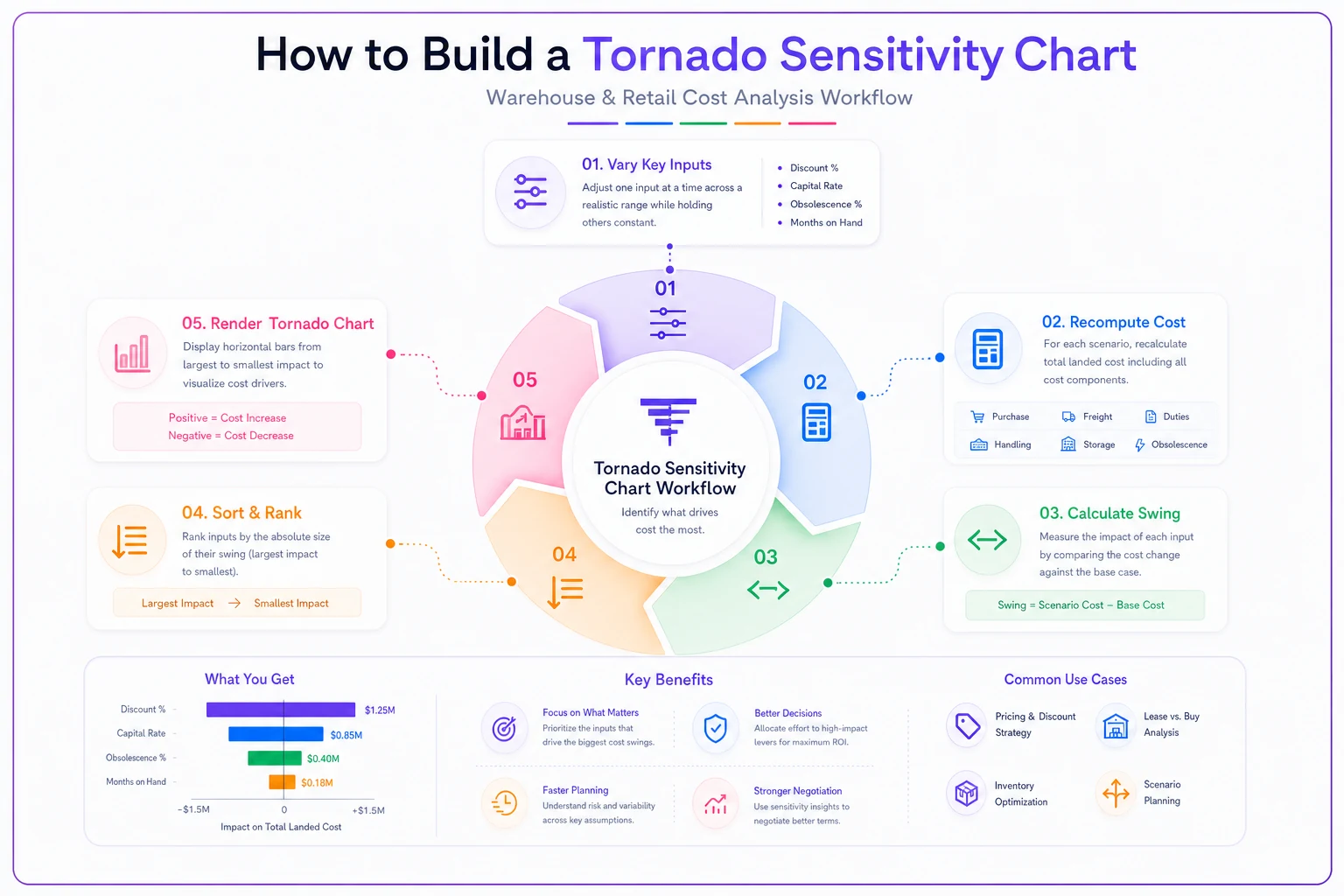
A compact diagram of the steps helps people see which assumptions to lock down first.
In most SMB pre‑buys, the two longest bars tend to be the capital rate and the obsolescence reserve — precisely the two numbers teams guess at. The freight premium matters less than people fear; the cost of cash and the risk of dead stock matter more.
Two‑way data table (Excel/Sheets):
Build a small grid with discount % down the left and capital rate across the top. In the top‑left corner cell, reference your total‑landed‑cost output. Then in Excel use Data → What‑If → Data Table (row input = capital rate cell, column input = discount cell). In Sheets, there's no native data table, so just lay out the grid and write a formula in each cell that recomputes landed cost for that pair — tedious but fast enough for a 5×5.
Reading it is the point: you'll find a diagonal boundary where full buy stops beating split buy. If your realistic assumptions sit near that boundary, don't over‑commit. Split.
Three‑tranche decision rules (shareable)
Once the model points toward splitting, you need rules the buyer can act on without re‑running math every time. These are worth printing out:
-
Tranche 1 (commit now) order 40–50% of projected season demand. Enough to lock the discount tier and cover the lead‑time window.
-
Tranche 2 (release trigger) place when sell‑through hits 35–40% of tranche 1, OR when you're inside the supplier's lead time for the peak window — whichever comes first.
-
Tranche 3 (confirm or cancel) decide at 65–70% sell‑through of tranches 1+2. If velocity is tracking at or above forecast, release it. If it's lagging more than ~15% under forecast, cancel or cut it in half.
-
Hard stop if obsolescence risk (seasonality, version change, expiry) lands within the horizon of tranche 3's expected hold time, don't place tranche 3 regardless of the discount.
These triggers are why split buys win on risk even when they lose a little on unit price: you get two chances to not buy the stuff that isn't selling.
Operational execution checklist
A model that lives in one person's laptop doesn't change anything. Assign it.
-
[ ] Owner
Buyer
— Inputs tab reviewed and updated with current freight, discount tiers, and the real capital rate (not the lazy one). Before every pre‑buy. -
[ ] Owner
Finance
— confirm the capital cost rate in B11 each quarter. This single cell shifts the whole decision. -
[ ] Owner
Warehouse lead
— confirm storage cost and that the units‑per‑pallet figure is current (packaging changes break this quietly). -
[ ] Owner
Buyer
— tranche 1 PO placed, tranche 2 and 3 set as draft POs with trigger dates and sell‑through thresholds noted on each. -
[ ] Owner
Inventory manager
— weekly sell‑through check against tranche triggers during the season. Flag at 35% and 65% marks. -
[ ] Deadline discipline tranche 2 decision logged no later than the trigger date — not "when we get to it." A missed release date turns a planned split into an emergency full‑price reorder.
-
[ ] Owner
Finance
— post‑season, compare actual landed cost per unit to the model's prediction. Feed the variance back into next year's assumptions.
That last step is where the model gets sharp. The first version of your sheet will be wrong on obsolescence and probably optimistic on sell‑through. One season of actuals fixes most of it.
When this model actually helps — and when it doesn't
It helps when: you're committing real cash to a pre‑buy, the discount is tempting, and you've got storage or cash constraints. Anything seasonal, anything with a version or expiry clock, anything where a wrong guess ties up five figures for months.
-
you're committing real cash to a pre‑buy, the discount is tempting, and you've got storage or cash constraints.
-
anything seasonal, anything with a version or expiry clock.
-
anything where a wrong guess ties up five figures for months.
It's overkill when: the buy is small, fast‑moving, and cheap to reorder. If the whole order turns in three weeks and reordering costs a phone call, don't build a tornado chart. Just buy it.
-
the buy is small, fast‑moving, and cheap to reorder.
Who should not lean on this: anyone who won't maintain the capital rate and obsolescence inputs honestly. A pre‑buy spreadsheet with stale assumptions is more dangerous than no model, because it hands you false confidence with a clean‑looking total.
A short note on accounting and tax
Two things worth a quick word with whoever does your books. First, that obsolescence reserve line in the model is a planning number — it's not the same as a booked inventory write‑down, and you can't deduct a reserve you've only estimated. The tax deduction comes when stock is actually written off or sold below cost.
Second, large pre‑buys shift when costs hit your books; under most inventory accounting the cost sits on the balance sheet until the unit sells, so a big December pre‑buy doesn't give you the expense in that year that some owners expect. Model the cash flow and the P&L timing separately — they aren't the same, and the difference has caught more than a few buyers off guard at year‑end.
Useful free tools to pair with the sheet
A few genuinely helpful free resources to speed up the inputs:
-
Pallet / cube converters search for a "freight density calculator" or "pallet dimensional weight calculator" — most major LTL carriers publish free ones that convert dimensions to pallet positions and cube.
-
Inventory / EOQ calculators free economic order quantity calculators are easy to find and give you a sanity check on order frequency, which maps directly to your B13–B15 inputs.
-
Carrying‑cost estimators several inventory blogs host free carrying‑cost calculators — useful for pressure‑testing your storage and capital lines if you don't have firm numbers yet.
Use these to populate the Inputs tab faster, then let your own all‑in per‑unit row make the call.
Wrapping up
The reason most pre‑buys go sideways isn't bad negotiation — it's a comparison that stops at the discount. The discount is real money, but so is the cash tied up for six months, the freight premium on split loads, the labor to receive and put away, and the slice of the lot that quietly goes stale. Put all of it in one sheet, point three strategies at it, and the right answer tends to show up on its own.
Build the three tabs. Fill in your honest numbers — especially the cost of cash. Run the two‑way table. Wire the tranche triggers to real sell‑through checks so the plan survives contact with an actual season. That's the whole system, and it fits in one spreadsheet.
Ready to optimize your inventory operations?
Join 2,000+ businesses using Listoly to reduce stockouts, save time, and improve order accuracy.